数据可视化matplotlib

import matplotlib.pyplot as pltimport numpy as np
import numpy.random as randn
import pandas as pd
from pandas import Series,DataFrame
from pylab import mpl
mpl.rcParams['axes.unicode_minus'] = False # 我自己配置的问题
plt.rc('figure', figsize=(10, 6)) # 设置图像大小
%matplotlib inline
1. figure对象
Matplotlib的图像均位于figure对象中。
创建figure: plt.figure()
fig = plt.figure()
2. subplot子图
add_subplot:向figure对象中添加子图。
add_subplot(a, b, c):a,b 表示讲fig分割成axb的区域,c 表示当前选中要操作的区域(c从1开始)。
add_subplot返回的是AxesSubplot对象,plot 绘图的区域是最后一次指定subplot的位置
ax1 = fig.add_subplot(2,2,1)ax2 = fig.add_subplot(2,2,2)
ax3 = fig.add_subplot(2,2,3)
ax4 = fig.add_subplot(2,2,4)
random_arr = randn.rand(50)# 默认是在最后一次使用subplot的位置上作图
plt.plot(random_arr,'ro--') # r:表示颜色为红色,o:表示数据用o标记 ,--:表示虚线
# 等价于:
# plt.plot(random_arr,linestyle='--',color='r',marker='o')
plt.show()
# hist:直方图:统计分布情况plt.hist(np.random.rand(8), bins=6, color='b', alpha=0.3)
# bins:数据箱子个数
(array([ 3., 0., 0., 0., 2., 3.]),array([ 0.10261627, 0.19557319, 0.28853011, 0.38148703, 0.47444396,
0.56740088, 0.6603578 ]),
<a list of 6 Patch objects>)
# 散点图plt.scatter(np.arange(30), np.arange(30) + 3 * randn.randn(30))
subplots :生成子图/子图数组
# 柱状图fig, ax = plt.subplots()
x = np.arange(5)
y1, y2 = np.random.randint(1, 25, size=(2, 5))
width = 0.25
ax.bar(x, y1, width, color='r')
# 画柱子ax.bar(x+width, y2, width, color='g')
# 画柱子ax.set_xticks(x+width)
ax.set_xticklabels(['a', 'b', 'c', 'd', 'e']) # 下标注明
fig, axes = plt.subplots(2, 2, sharex=True, sharey=True) # 共享轴坐标
subplots_adjust:调整subplots的间距
plt.subplots_adjust(left=0.5,top=0.5)
fig, axes = plt.subplots(2, 2)
random_arr = randn.randn(8)fig, axes = plt.subplots(2, 2)
axes[0, 0].hist(random_arr, bins=16, color='k', alpha=0.5)
axes[0, 1].plot(random_arr,'ko--')
x = np.arange(8)
y = x + 5 * np.random.rand(8)
axes[1,0].scatter(x, y)
x = np.arange(5)
y1, y2 = np.random.randint(1, 25, size=(2, 5))
width = 0.25axes[1,1].bar(x, y1, width, color='r') # 画柱子
axes[1,1].bar(x+width, y2, width, color='g') # 画柱子
axes[1,1].set_xticks(x+width)
axes[1,1].set_xticklabels(['a', 'b', 'c', 'd', 'e']) # 下标注明
重叠绘制
legend:显示图例
random_arr1 = randn.randn(8)
random_arr2 = randn.randn(8)
fig, ax = plt.subplots()ax.plot(random_arr1,'ko--',label='A')
ax.plot(random_arr2,'b^--',label='B')
plt.legend(loc='best') # 自动选择放置图例的最佳位置
设置刻度范围:set_xlim、set_ylim
设置显示的刻度:set_xticks、set_yticks
刻度标签:set_xticklabels、set_yticklabels
坐标轴标签:set_xlabel、set_ylabe
l图像标题:set_title
fig, ax = plt.subplots(1)ax.plot(np.random.randn(380).cumsum())
# 设置刻度范围a
x.set_xlim([0, 500])
# 设置显示的刻度(记号)
ax.set_xticks(range(0,500,100))
# 设置刻度标签
ax.set_xticklabels(['one', 'two', 'three', 'four', 'five'],
rotation=30, fontsize='small')
# 设置坐标轴标签ax.set_xlabel('X:...')
ax.set_ylabel('Y:...')
# 设置标题
ax.set_title('Example')
3. Plotting functions in pandas
plt.close('all')s = Series(np.random.randn(10).cumsum(), index=np.arange(0, 100, 10))
s
fig,ax = plt.subplots(1)
s.plot(ax=ax,style='ko--')
fig, axes = plt.subplots(2, 1)data = Series(np.random.rand(16), index=list('abcdefghijklmnop'))
data.plot(kind='bar', ax=axes[0], color='k', alpha=0.7)
data.plot(kind='barh', ax=axes[1], color='k', alpha=0.7)
df = DataFrame(np.random.randn(10, 4).cumsum(0),columns=['A', 'B', 'C', 'D'],
index=np.arange(0, 100, 10))
df
df.plot() # 列索引为图例,行索引为横坐标,值为纵坐标
df = DataFrame(np.random.randint(0,2,(10, 2)),columns=['A', 'B'],
index=np.arange(0, 10, 1))
df
df.plot(kind='bar')
df.A.value_counts().plot(kind='bar')
df.A[df.B == 1].plot(kind='kde')df.A[df.B == 0].plot(kind='kde') # 密度图
df = DataFrame(np.random.rand(6, 4),index=['one', 'two', 'three', 'four', 'five', 'six'],
columns=pd.Index(['A', 'B', 'C', 'D'], name='Genus'))
df
df.plot(kind='bar',stacked='True') #行索引:横坐标
values = Series(np.random.normal(0, 1, size=200))values.hist(bins=100, alpha=0.3, color='k', normed=True)
values.plot(kind='kde', style='k--')
df = DataFrame(np.random.randn(10,2),columns=['A', 'B'],
index=np.arange(0, 10, 1))
df
plt.scatter(df.A, df.B)
更多python相关文章请关注python自学网。
以上是 数据可视化matplotlib 的全部内容, 来源链接: utcz.com/z/540949.html