浅谈pytorch中torch.max和F.softmax函数的维度解释
在利用torch.max函数和F.Ssoftmax函数" title="softmax函数">softmax函数时,对应该设置什么维度,总是有点懵,遂总结一下:
首先看看二维tensor的函数的例子:
import torch
import torch.nn.functional as F
input = torch.randn(3,4)
print(input)
tensor([[-0.5526, -0.0194, 2.1469, -0.2567],
[-0.3337, -0.9229, 0.0376, -0.0801],
[ 1.4721, 0.1181, -2.6214, 1.7721]])
b = F.softmax(input,dim=0) # 按列SoftMax,列和为1
print(b)
tensor([[0.1018, 0.3918, 0.8851, 0.1021],
[0.1268, 0.1587, 0.1074, 0.1218],
[0.7714, 0.4495, 0.0075, 0.7762]])
c = F.softmax(input,dim=1) # 按行SoftMax,行和为1
print(c)
tensor([[0.0529, 0.0901, 0.7860, 0.0710],
[0.2329, 0.1292, 0.3377, 0.3002],
[0.3810, 0.0984, 0.0064, 0.5143]])
d = torch.max(input,dim=0) # 按列取max,
print(d)
torch.return_types.max(
values=tensor([1.4721, 0.1181, 2.1469, 1.7721]),
indices=tensor([2, 2, 0, 2]))
e = torch.max(input,dim=1) # 按行取max,
print(e)
torch.return_types.max(
values=tensor([2.1469, 0.0376, 1.7721]),
indices=tensor([2, 2, 3]))
下面看看三维tensor解释例子:
函数softmax输出的是所给矩阵的概率分布;
b输出的是在dim=0维上的概率分布,b[0][5][6]+b[1][5][6]+b[2][5][6]=1
a=torch.rand(3,16,20)
b=F.softmax(a,dim=0)
c=F.softmax(a,dim=1)
d=F.softmax(a,dim=2)
In [1]: import torch as t
In [2]: import torch.nn.functional as F
In [4]: a=t.Tensor(3,4,5)
In [5]: b=F.softmax(a,dim=0)
In [6]: c=F.softmax(a,dim=1)
In [7]: d=F.softmax(a,dim=2)
In [8]: a
Out[8]:
tensor([[[-0.1581, 0.0000, 0.0000, 0.0000, -0.0344],
[ 0.0000, -0.0344, 0.0000, -0.0344, 0.0000],
[-0.0344, 0.0000, -0.0344, 0.0000, -0.0344],
[ 0.0000, -0.0344, 0.0000, -0.0344, 0.0000]],
[[-0.0344, 0.0000, -0.0344, 0.0000, -0.0344],
[ 0.0000, -0.0344, 0.0000, -0.0344, 0.0000],
[-0.0344, 0.0000, -0.0344, 0.0000, -0.0344],
[ 0.0000, -0.0344, 0.0000, -0.0344, 0.0000]],
[[-0.0344, 0.0000, -0.0344, 0.0000, -0.0344],
[ 0.0000, -0.0344, 0.0000, -0.0344, 0.0000],
[-0.0344, 0.0000, -0.0344, 0.0000, -0.0344],
[ 0.0000, -0.0344, 0.0000, -0.0344, 0.0000]]])
In [9]: b
Out[9]:
tensor([[[0.3064, 0.3333, 0.3410, 0.3333, 0.3333],
[0.3333, 0.3333, 0.3333, 0.3333, 0.3333],
[0.3333, 0.3333, 0.3333, 0.3333, 0.3333],
[0.3333, 0.3333, 0.3333, 0.3333, 0.3333]],
[[0.3468, 0.3333, 0.3295, 0.3333, 0.3333],
[0.3333, 0.3333, 0.3333, 0.3333, 0.3333],
[0.3333, 0.3333, 0.3333, 0.3333, 0.3333],
[0.3333, 0.3333, 0.3333, 0.3333, 0.3333]],
[[0.3468, 0.3333, 0.3295, 0.3333, 0.3333],
[0.3333, 0.3333, 0.3333, 0.3333, 0.3333],
[0.3333, 0.3333, 0.3333, 0.3333, 0.3333],
[0.3333, 0.3333, 0.3333, 0.3333, 0.3333]]])
In [10]: b.sum()
Out[10]: tensor(20.0000)
In [11]: b[0][0][0]+b[1][0][0]+b[2][0][0]
Out[11]: tensor(1.0000)
In [12]: c.sum()
Out[12]: tensor(15.)
In [13]: c
Out[13]:
tensor([[[0.2235, 0.2543, 0.2521, 0.2543, 0.2457],
[0.2618, 0.2457, 0.2521, 0.2457, 0.2543],
[0.2529, 0.2543, 0.2436, 0.2543, 0.2457],
[0.2618, 0.2457, 0.2521, 0.2457, 0.2543]],
[[0.2457, 0.2543, 0.2457, 0.2543, 0.2457],
[0.2543, 0.2457, 0.2543, 0.2457, 0.2543],
[0.2457, 0.2543, 0.2457, 0.2543, 0.2457],
[0.2543, 0.2457, 0.2543, 0.2457, 0.2543]],
[[0.2457, 0.2543, 0.2457, 0.2543, 0.2457],
[0.2543, 0.2457, 0.2543, 0.2457, 0.2543],
[0.2457, 0.2543, 0.2457, 0.2543, 0.2457],
[0.2543, 0.2457, 0.2543, 0.2457, 0.2543]]])
In [14]: n=t.rand(3,4)
In [15]: n
Out[15]:
tensor([[0.2769, 0.3475, 0.8914, 0.6845],
[0.9251, 0.3976, 0.8690, 0.4510],
[0.8249, 0.1157, 0.3075, 0.3799]])
In [16]: m=t.argmax(n,dim=0)
In [17]: m
Out[17]: tensor([1, 1, 0, 0])
In [18]: p=t.argmax(n,dim=1)
In [19]: p
Out[19]: tensor([2, 0, 0])
In [20]: d.sum()
Out[20]: tensor(12.0000)
In [22]: d
Out[22]:
tensor([[[0.1771, 0.2075, 0.2075, 0.2075, 0.2005],
[0.2027, 0.1959, 0.2027, 0.1959, 0.2027],
[0.1972, 0.2041, 0.1972, 0.2041, 0.1972],
[0.2027, 0.1959, 0.2027, 0.1959, 0.2027]],
[[0.1972, 0.2041, 0.1972, 0.2041, 0.1972],
[0.2027, 0.1959, 0.2027, 0.1959, 0.2027],
[0.1972, 0.2041, 0.1972, 0.2041, 0.1972],
[0.2027, 0.1959, 0.2027, 0.1959, 0.2027]],
[[0.1972, 0.2041, 0.1972, 0.2041, 0.1972],
[0.2027, 0.1959, 0.2027, 0.1959, 0.2027],
[0.1972, 0.2041, 0.1972, 0.2041, 0.1972],
[0.2027, 0.1959, 0.2027, 0.1959, 0.2027]]])
In [23]: d[0][0].sum()
Out[23]: tensor(1.)
补充知识:多分类问题torch.nn.Softmax的使用
为什么谈论这个问题呢?是因为我在工作的过程中遇到了语义分割预测输出特征图个数为16,也就是所谓的16分类问题。
因为每个通道的像素的值的大小代表了像素属于该通道的类的大小,为了在一张图上用不同的颜色显示出来,我不得不学习了torch.nn.Softmax的使用。
首先看一个简答的例子,倘若输出为(3, 4, 4),也就是3张4x4的特征图。
import torch
img = torch.rand((3,4,4))
print(img)
输出为:
tensor([[[0.0413, 0.8728, 0.8926, 0.0693],
[0.4072, 0.0302, 0.9248, 0.6676],
[0.4699, 0.9197, 0.3333, 0.4809],
[0.3877, 0.7673, 0.6132, 0.5203]],
[[0.4940, 0.7996, 0.5513, 0.8016],
[0.1157, 0.8323, 0.9944, 0.2127],
[0.3055, 0.4343, 0.8123, 0.3184],
[0.8246, 0.6731, 0.3229, 0.1730]],
[[0.0661, 0.1905, 0.4490, 0.7484],
[0.4013, 0.1468, 0.2145, 0.8838],
[0.0083, 0.5029, 0.0141, 0.8998],
[0.8673, 0.2308, 0.8808, 0.0532]]])
我们可以看到共三张特征图,每张特征图上对应的值越大,说明属于该特征图对应类的概率越大。
import torch.nn as nn
sogtmax = nn.Softmax(dim=0)
img = sogtmax(img)
print(img)
输出为:
tensor([[[0.2780, 0.4107, 0.4251, 0.1979],
[0.3648, 0.2297, 0.3901, 0.3477],
[0.4035, 0.4396, 0.2993, 0.2967],
[0.2402, 0.4008, 0.3273, 0.4285]],
[[0.4371, 0.3817, 0.3022, 0.4117],
[0.2726, 0.5122, 0.4182, 0.2206],
[0.3423, 0.2706, 0.4832, 0.2522],
[0.3718, 0.3648, 0.2449, 0.3028]],
[[0.2849, 0.2076, 0.2728, 0.3904],
[0.3627, 0.2581, 0.1917, 0.4317],
[0.2543, 0.2898, 0.2175, 0.4511],
[0.3880, 0.2344, 0.4278, 0.2686]]])
可以看到,上面的代码对每张特征图对应位置的像素值进行Softmax函数处理, 图中标红位置加和=1,同理,标蓝位置加和=1。
我们看到Softmax函数会对原特征图每个像素的值在对应维度(这里dim=0,也就是第一维)上进行计算,将其处理到0~1之间,并且大小固定不变。
print(torch.max(img,0))
输出为:
torch.return_types.max(
values=tensor([[0.4371, 0.4107, 0.4251, 0.4117],
[0.3648, 0.5122, 0.4182, 0.4317],
[0.4035, 0.4396, 0.4832, 0.4511],
[0.3880, 0.4008, 0.4278, 0.4285]]),
indices=tensor([[1, 0, 0, 1],
[0, 1, 1, 2],
[0, 0, 1, 2],
[2, 0, 2, 0]]))
可以看到这里3x4x4变成了1x4x4,而且对应位置上的值为像素对应每个通道上的最大值,并且indices是对应的分类。
清楚理解了上面的流程,那么我们就容易处理了。
看具体案例,这里输出output的大小为:16x416x416.
output = torch.tensor(output)
sm = nn.Softmax(dim=0)
output = sm(output)
mask = torch.max(output,0).indices.numpy()
# 因为要转化为RGB彩色图,所以增加一维
rgb_img = np.zeros((output.shape[1], output.shape[2], 3))
for i in range(len(mask)):
for j in range(len(mask[0])):
if mask[i][j] == 0:
rgb_img[i][j][0] = 255
rgb_img[i][j][1] = 255
rgb_img[i][j][2] = 255
if mask[i][j] == 1:
rgb_img[i][j][0] = 255
rgb_img[i][j][1] = 180
rgb_img[i][j][2] = 0
if mask[i][j] == 2:
rgb_img[i][j][0] = 255
rgb_img[i][j][1] = 180
rgb_img[i][j][2] = 180
if mask[i][j] == 3:
rgb_img[i][j][0] = 255
rgb_img[i][j][1] = 180
rgb_img[i][j][2] = 255
if mask[i][j] == 4:
rgb_img[i][j][0] = 255
rgb_img[i][j][1] = 255
rgb_img[i][j][2] = 180
if mask[i][j] == 5:
rgb_img[i][j][0] = 255
rgb_img[i][j][1] = 255
rgb_img[i][j][2] = 0
if mask[i][j] == 6:
rgb_img[i][j][0] = 255
rgb_img[i][j][1] = 0
rgb_img[i][j][2] = 180
if mask[i][j] == 7:
rgb_img[i][j][0] = 255
rgb_img[i][j][1] = 0
rgb_img[i][j][2] = 255
if mask[i][j] == 8:
rgb_img[i][j][0] = 255
rgb_img[i][j][1] = 0
rgb_img[i][j][2] = 0
if mask[i][j] == 9:
rgb_img[i][j][0] = 180
rgb_img[i][j][1] = 0
rgb_img[i][j][2] = 0
if mask[i][j] == 10:
rgb_img[i][j][0] = 180
rgb_img[i][j][1] = 255
rgb_img[i][j][2] = 255
if mask[i][j] == 11:
rgb_img[i][j][0] = 180
rgb_img[i][j][1] = 0
rgb_img[i][j][2] = 180
if mask[i][j] == 12:
rgb_img[i][j][0] = 180
rgb_img[i][j][1] = 0
rgb_img[i][j][2] = 255
if mask[i][j] == 13:
rgb_img[i][j][0] = 180
rgb_img[i][j][1] = 255
rgb_img[i][j][2] = 180
if mask[i][j] == 14:
rgb_img[i][j][0] = 0
rgb_img[i][j][1] = 180
rgb_img[i][j][2] = 255
if mask[i][j] == 15:
rgb_img[i][j][0] = 0
rgb_img[i][j][1] = 0
rgb_img[i][j][2] = 0
cv2.imwrite('output.jpg', rgb_img)
最后保存得到的图为:
以上这篇浅谈pytorch中torch.max和F.softmax函数的维度解释就是小编分享给大家的全部内容了,希望能给大家一个参考,也希望大家多多支持。
以上是 浅谈pytorch中torch.max和F.softmax函数的维度解释 的全部内容, 来源链接: utcz.com/z/332189.html